Usage

The base classes to access bursts, burst observations, and burst sources are minbar.Bursts, minbar.Observations, and minbar.Sources, respectively. Creating instances of each one will read the data from the corresponding table file.

Here we provide basic usage; more examples are provided in the tutorial jupyter notebook

1. Working with bursts

Here we initialise a minbar.Bursts object, and select all the bursts from 4U 1636-536

import minbar
mb = minbar.Bursts() # Load the burst database
mb.name_like('1636') # Select a source using part of its name
print (mb.field_labels.keys()) # See which fields are available
mb.show() # List the selected bursts

The selection made with the minbar.Minbar.name_like() and equivalent commands is persistent, and any subsequent query (e.g. extracting one of the table columns) will be restricted to the same set of events. You can reset to the full sample with minbar.Minbar.clear()

Let’s explore that below with some slightly more complex includes and excludes

mb.clear() # Reset the selection
mb.select_all(['GS 1826-24', '4U 1636-536']) # Select multiple sources; requires exact names
mb.clear() # Clear the selection so all sources are included
mb.exclude_like('1636') # Exclude source from selection
mb.exclude_like('1826') # Now two sources are excluded

Here’s some analysis which involves working with the fluxes, and estimating peak luminosity from the bolometric peak flux (table attribute bpflux)

time = mb['time'] # Get a field as a numpy array (automatically time-ordered)
id = mb[time > 54000.]['entry'] # extract ID #s for all the bursts after the specified time
flux = mb['bpflux'] # Flux in 1e-9 erg/s/cm2
sub = mb[['time','bpflux']] # extract a subset of the columns, for the given selection
mb.create_distance_correction() # Include distance information from Sources()
luminosity = (flux*mb['distcor']).to('erg s-1') # Isotropic peak luminosity in erg/s
pca = mb.instr_like('pca') # Get index array for bursts observed with PCA
pca_luminosity = luminosity[pca] # Luminosity of PCA bursts

A complete list of the minbar.Bursts table attributes, along with those for the Observations and Sources tables, can be found at the alternate web interface for the MINBAR data, http://burst.sci.monash.edu

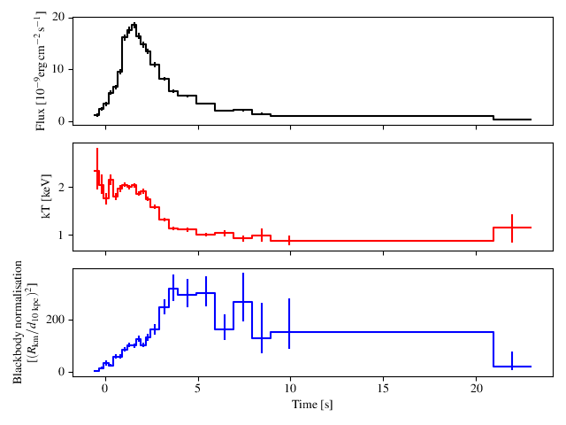
Time-resolved spectroscopy for most of the RXTE/PCA and BeppoSAX/WFC bursts is available via the website, but can be downloaded using the minbar.Bursts.get_burst_data() method. The minbar.Bursts.burstplot() method can make nice plots of the downloaded data, or will just download the data on request as needed:

print (mb[2258]) # show the data table row for the 2nd burst from obsID 10088-01-07-02
data = mb.get_burst_data(2258) # download the time-resolved spectroscopy table
data.columns # show the available columns
mb.burstplot(bdata=data) # plot those data, default is flux only
mb.burstplot(2258, param=['flux','kT','rad']) # download and plot in one step, with extra parameters

The result of the last command is shown below; from top to bottom, bolometric burst flux, blackbody temperature, and radius. Use the show=False option to minbar.Bursts.burstplot() to add your own annotation before calling plt.show().

2. Working with observations

As both the minbar.Bursts and minbar.Observations classes are built on the underlying minbar.Minbar class, many of the methods are common to both classes.

Below whe show an example of selecting all the observations from 4U 1636-536 and extracting the start times.

mo = minbar.Observations() # Load the observation database
mo.name_like('1636') # Same source selection options as for burst database
time = mo['tstart'] # And fields are accessed in the same way
print (mo.field_labels.keys()) # See which fields are available

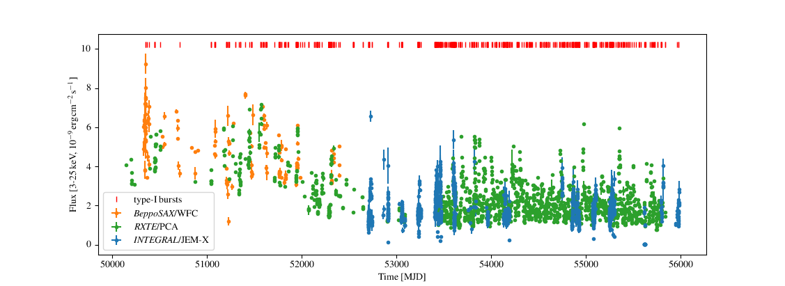
We can also plot the long-term history of the source using the plot method, first selecting only the “good” observations (non-zero fluxes, principally)

mo.good()
mo.plot()

The result is below

3. Working with sources

The minbar.Sources class is a little different as it is really just a wrapper for the underlying FITS table. Still, some of the methods as for the other two classes are available, including minbar.Sources.name_like().

Note that available minbar.Sources methods do not include select_all or exclude_like

You can also select sources by type, e.g. C for ultracompact, or S for sources that have shown a superburst, or combinations of the two

ms = minbar.Sources() # Load the source database
print (ms.field_labels.keys()) # Show available data fields
ra = ms['ra_obj'] # Right ascension for all sources
ms.name_like('1636') # Select a source using part of its name
ra = ms['ra_obj'] # Right ascension for selected source only
ms.clear() # Clear selection
ms.type('SC') # Select all ultracompacts that have shown a superburst
ms['name'] # ... and show their names

4. Analysing new X-ray observations

Below are some basic examples to analyse some (new?) X-ray data and search for bursts (under development)

import minbar

xte = minbar.Instrument('PCA') # Create an instrument definition
obs = minbar.Observation(None, xte, '4U 1636-536', '10088-01-07-02')

obs.plot()
print (obs.mjd, obs.rate)

Can also define a new instrument for analysis of data from instruments not originally part of MINBAR

xmm = minbar.Instrument('XMM-Newton', 'xmm', 'XN', '2to7good.fits')
obs = minbar.Observation(None, xmm, '1RXS J180408.9-342058', '0741620101')
lc =obs.get_lc()

import matplotlib.pyplot as plt
plt.plot(lc['TIME'], lc['RATE'])
plt.show()

And search for bursts

test = minbar.findburst(lc['TIME'], lc['RATE'], lc['ERROR'])
print(test)
[5.42058957e+08 5.42067368e+08 5.42075296e+08 5.42083081e+08
 5.42090903e+08]

These tools are currently under development